Although we have the desired result (4.39), let us note that there is another way of deriving it, which is often easier than direct application of (4.3). The principle was introduced in our derivation of (3.33): resolve the proposition whose probability is desired (in this case D) into mutually exclusive propositions, and calculate the sum of their probabilities. We can carry out this resolution in many different ways by ‘introducing into the conversation’ any set of mutually exclusive and exhaustive propositions {P, Q, R, . . .} and using the rules of Boolean algebra:

虽然我们得到了理想的结果（4.39），但是让我们注意到有另一种推导它的方法，这通常比直接应用（4.3）更容易。 在我们推导的（3.33）中引入了这个原理：将需要概率的命题（在这种情况下为D）解析为互斥命题，并计算它们的概率之和。 我们可以通过“在会话中引入”任何一组相互排斥和详尽的命题{P，Q，R，…​}，以多种不同方式执行这一决议。。 。}并使用布尔代数的规则：

But the success of the method depends on our cleverness at choosing a particular set for which we can complete the calculation. This means that the propositions introduced must have a known kind of relevance to the question being asked; the example of penguins at the end of Chapter 2 will not be helpful if that question has nothing to do with penguins.

但是该方法的成功取决于我们选择特定集合的聪明程度，我们可以完成计算。 这意味着所引入的命题必须与所提出的问题具有已知类型的相关性; 如果这个问题与企鹅无关，那么第2章末尾的企鹅的例子将无济于事。

In the present case, for evaluation of $P(D|\bar{C}X)$, it appears that propositions A and B have this kind of relevance. Again, we note that proposition $\bar{C}$ implies (A + B); and so

在本案例中，对于$P（D | \ bar {C} X）$的评估，似乎命题A和B具有这种相关性。 同样，我们注意到命题$\ bar {C}$暗示（A + B）; 所以

These probabilities can be factored by the product rule:

But we can abbreviate: $P(D|A\bar{C}X) ≡ P(D|AX)$ and $P(D|B\bar{C}X) ≡ P(D|BX)$, because, in the way we set up this problem, the statement that either A or B is true implies that C must be false. For this same reason, P(\bar{C}|AX) = 1, and so, by the product rule,

and similarly for $P(B|\bar{C}X)$. Substituting these results into (4.42) and using (4.37), we again arrive at (4.39). This agreement provides another illustration – and a rather severe test – of the consistency of our rules for extended logic.

Returning to (4.39), we have the numerical value

and everything in (4.33) is now at hand. If we put all these things together, we find that the evidence for proposition C is:

If m > 5, a good approximation is

and if m < 3, a crude approximation is

Proposition C starts out at −60 db, and the first few bad widgets we find will each give about 7.73 db of evidence in favor of C, so the graph of e(C|DX) vs. m will start upward at a slope of 7.73. But then the slope drops, when m > 5, to 4.73. The evidence for C reaches 0 db when $m \simeq 49.6/4.73 = 10.5$. So, ten consecutive bad widgets would be enough to raise this initially very improbable hypothesis by 58 db, to the place where the robot is ready to consider it very seriously; and 11 consecutive bad ones would take it over the threshold, to where the robot considers it more likely to be true than false.

命题C从-60 db开始，我们找到的前几个坏小部件每个都会给出大约7.73 db的证据支持C，因此e（C | DX）与m的关系图将以一个斜率向上开始7.73。但是当m> 5时，斜率下降到4.73。当$m \ simeq 49.6 / 4.73 = 10.5$时，C的证据达到0 db。因此，十个连续的坏小部件足以将这个最初非常不可能的假设提高到58分贝到机器人准备好认真对待的地方;并且11个连续的坏的将超过阈值，机器人认为它更可能是真假而不是假。

In the meantime, what is happening to our propositions A and B? As before, A starts off at −10 db, B starts off at +10 db, and the plausibility for A starts going up 3 db per defective widget. But after we’ve found too many bad ones, that skepticism would set in, and you and I would begin to doubt whether the evidence really supports proposition A after all; proposition C is becoming a much easier way to explain what is observed. Has the robot also learned to be skeptical?

与此同时，我们的命题A和B发生了什么？和以前一样，A从-10 db开始，B从+10 db开始，A的合理性开始上升3 db每个有缺陷的widget。但是，在我们发现了太多不好的东西后，怀疑论就会出现，你和我会开始怀疑证据是否真的支持命题A;命题C正在变得更容易解释观察到的内容。机器人是否也学会了持怀疑态度？

After m widgets have been tested, and all proved to be bad, the evidence for propositions A and B, and the approximate forms, are as follows:

在测试了m小部件后，所有小部件都被证明是坏的，命题A和B的证据以及近似形式如下：

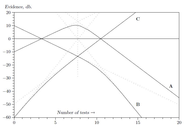
Fig. 4.1. A surprising multiple sequential test wherein a dead hypothesis © is resurrected.

The exact results are summarized in Figure 4.1. We can learn quite a lot about multiple hypothesis testing from studying this diagram. The initial straight line part of the A and B curves represents the solution as we found it before we introduced proposition C; the change in plausibility for propositions A and B starts off just the same as in the previous problem. The effect of proposition C does not appear until we have reached the place where C crosses B. At this point, suddenly the character of the A curve changes; instead of going on up, at m = 7 it has reached its highest value of 10 db. Then it turns around and comes back down; the robot has indeed learned how to become skeptical. But the B curve does not change at this point; it continues on linearly until it reaches the place where A and C have the same plausibility, and at this point it has a change in slope. From then on, it falls off more rapidly.

确切的结果总结在图4.1中。通过研究该图，我们可以从多个假设检验中学到很多东西。 A和B曲线的初始直线部分代表我们在引入命题C之前发现的解;命题A和B的合理性变化与前一个问题的开始时相同。直到我们到达C穿过B的地方才出现命题C的效果。此时，A曲线的特征突然改变;而不是继续上升，在m = 7时它达到了10分贝的最高值。然后它转过身来回来;机器人确实学会了如何变得持怀疑态度。但是B曲线此时并没有改变;它继续线性地直到它到达A和C具有相同合理性的地方，并且此时它具有斜率的变化。从那时起，它会更快地下降。

Most people find all this surprising and mysterious at first glance; but then a little meditation is enough to make us perceive what is happening and why. The change in plausibility for A due to one more test arises from the fact that we are now testing hypothesis A against two alternatives: B and C. But, initially, B is so much more plausible than C, that for all practical purposes we are simply testing A against B, and reproducing our previous solution (4.22). After enough evidence has accumulated to bring the plausibility for C up to the same level as B, then from that point on A is essentially being tested against C instead of B, which is a very different situation.

大多数人乍一看都发现这一切令人惊讶和神秘;但是，稍微冥想就足以让我们了解正在发生的事情和原因。由于再进行一次测试，A的合理性变化源于这样一个事实，即我们现在正在测试假设A对两种选择：B和​​C.但是，最初，B比C更合理，对于所有实际目的我们都是只需针对B测试A，并复制我们以前的解决方案（4.22）。在积累了足够的证据以使C的合理性达到与B相同的水平之后，从A点开始，A基本上是针对C而不是B进行测试，这是一种非常不同的情况。

All of these changes in slope can be interpreted in this way. Once we see this principle, it is clear that the same thing is going to be true more generally. As long as we have a discrete set of hypotheses, a change in plausibility for any one of them will be approximately the result of a test of this hypothesis against a single alternative – the single alternative being that one of the remaining hypotheses which is most plausible at that time. As the relative plausibilities of the alternatives change, the slope of the A curve must also change; this is the cogent information that would be lost if we tried to retain the independent additive form (4.13) when n > 2.

斜率的所有这些变化都可以这种方式解释。一旦我们看到这个原则，很明显同样的事情会更普遍地成为现实。只要我们有一组离散的假设，其中任何一个假设的合理性变化大约是对这个假设进行单一替代检验的结果 - 唯一的替代方案是其中一个最合理的假设那时候。随着替代方案的相对合理性发生变化，A曲线的斜率也必须改变;如果我们在n> 2时试图保留独立的添加剂形式（4.13），这将是有用的信息。

Whenever the hypotheses are separated by about 10 db or more, then multiple hypothesis testing reduces approximately to testing each hypothesis against a single alternative. So, seeing this, you can construct curves of the sort shown in Fig. 4.1 very rapidly without even writing down the equations, because what would happen in the two-hypothesis case is easily seen once and for all. The diagram has a number of other interesting geometrical properties, suggested by drawing the six asymptotes and noting their vertical alignment (dotted lines), which we leave for the reader to explore.

每当假设被分开大约10分贝或更多时，则多个假设检验大约减少以针对单个替代方案测试每个假设。因此，看到这一点，你可以非常快速地构建图4.1所示类型的曲线，甚至不用写下方程式，因为在两个假设情况下会发生的事情很容易一劳永逸地看到。该图有许多其他有趣的几何属性，通过绘制六个渐近线并注意它们的垂直对齐（虚线）来建议，我们留给读者探索。

All the information needed to construct fairly accurate charts resulting from any sequence of good and bad tests is contained in the ‘plausibility flow diagrams’ of Figure 4.2, which summarize the solutions of all those binary problems; every possible way to test one proposition against a single alternative. It indicates, for example, that finding a good widget raises the evidence for B by 1 db if B is being tested against A, and by 19.22 db if it is being tested against C. Similarly, finding a bad widget raises the evidence for A by 3 db if A is being tested against B, but lowers it by 4.73 db if it is being tested against C. Likewise, we see that finding a single good widget lowers the evidence for C by an amount that cannot be recovered by two bad ones; so there is a ‘threshold of skepticism’. C will never attain an appreciable probability; i.e. the robot will never become skeptical about propositions A and B, as long as the observed fraction f of bad ones remains less than 2/3.

构建相当准确的图表所需的所有信息都来自于图4.2的“合理性流程图”，它总结了所有这些二元问题的解决方案;一种可能的方法来测试一个命题与一个替代方案。例如，它表明，如果B正在针对A进行测试，那么找到一个好的窗口小部件会将B的证据提高1分贝，如果针对C进行测试则会提高19.22分贝。同样，找到一个坏窗口小部件会提高A的证据如果A正在针对B进行测试，那么通过3分贝进行测试，但是如果针对C进行测试则将其降低4.73分贝。同样，我们看到找到一个好的小部件可以将C的证据降低两个不能恢复的数量那些;所以有一个“怀疑的门槛”。 C永远不会达到明显的概率;即机器人永远不会对命题A和B持怀疑态度，只要观察到的坏分数f仍小于2/3。

More precisely,we define a threshold fraction ft thus: as the number of testsm →∞ with f = mb/m → const., e(C|DX) tends to +∞ if f > ft, and to −∞ if f < ft. The exact threshold turns out to be greater than 2/3: $f_t$ = 0.793951 (Exercise 4.2). If the observed

更准确地说，我们定义了一个阈值分数ft：当测试的数量为→∞，其中f = mb / m→const。，如果f> ft，则e（C | DX）倾向于+∞，如果f <，则为-∞ ft。确切的阈值大于2/3：$f_t$ = 0.793951（练习4.2）。如果观察到了

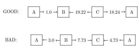
Fig. 4.2. Plausibility flow diagrams.

fraction of bad widgets remains above this value, the robot will be led eventually to prefer proposition C over A and B.

坏小部件的一部分仍然高于这个值，机器人将最终被引导优先于A和B的命题C.

Exercise 4.2. Calculate the exact threshold of skepticism ft(x, y), supposing that proposition C has instead of $10^{−6}$ an arbitrary prior probability P(C|X) = x, and specifies instead of 99/100 an arbitrary fraction y of bad widgets. Then discuss how the dependence on x and y corresponds – or fails to correspond – to human common sense.

练习4.2。 计算怀疑主义ft（x，y）的确切阈值，假设命题C代替$10 ^ { - 6}$任意先验概率P（C | X）= x，并指定而不是99/100 坏小部件的任意分数y。 然后讨论对x和y的依赖如何与人类常识相对应 - 或者不对应 - 。

Hint: In problems like this, always try first to get an analytic solution in closed form. If you are unable to do this, then you must write a short computer program which will display the correct numerical values in tables or graphs.

提示：在这样的问题中，总是先尝试以封闭的形式获得分析解决方案。 如果您无法执行此操作，则必须编写一个简短的计算机程序，该程序将在表格或图形中显示正确的数值。

Exercise 4.3. Show how to make the robot skeptical about both unexpectedly high and unexpectedly low numbers of bad widgets in the observed sample. Give the full equations. Note particularly the following: if A is true, then wewould expect, according to the binomial distribution (3.86), that the observed fraction of bad ones would tend to about 1/3 with many tests, while if B is true it should tend to 1/6. Suppose that it is found to tend to the threshold value (4.24), close to 1/4. On sufficiently large m, you and I would then become skeptical about A and B; but intuition tells us that this would require a much larger m than ten, which was enough to make us and the robot skeptical when we find them all bad. Do the equations agree with our intuition here, if a new hypothesis F is introduced which specifies P(bad|FX) $\simeq$ 1/4?

练习4.3。展示如何使机器人对观察到的样本中意外高和意外低数量的坏小部件持怀疑态度。给出完整的方程式。特别注意以下内容：如果A为真，那么根据二项式分布（3.86），我们可以预期，观察到的坏分数会在许多测试中趋于约1/3，而如果B为真，则应倾向于1/6。假设它发现倾向于阈值（4.24），接近1/4。在足够大的m上，你和我会对A和B持怀疑态度;但直觉告诉我们，这需要比10更大的m，这足以让我们和机器人在我们发现它们都很糟糕时持怀疑态度。如果引入一个新的假设F指定P（bad | FX）$\ simeq$ 1/4，这些方程式是否符合我们的直觉？

In summary, the role of our new hypothesis C was only to be held in abeyance until needed, like a fire extinguisher. In a normal testing situation it is ‘dead’, playing no part in the inference because its probability is and remains far below that of the other hypotheses. But a dead hypothesis can be resurrected to life by very unexpected data. Exercises 4.2 and 4.3 ask the reader to explore the phenomenon of resurrection of dead hypotheses in more detail than we do in this chapter, but we return to the subject in Chapter 5.

总之，我们的新假设C的作用只是在需要之前暂时搁置，就像灭火器一样。在正常的测试情况下，它是“死的”，不参与推理，因为它的概率是远远低于其他假设的概率。但是，一个死的假设可以通过非常意外的数据复活到生命中。练习4.2和4.3要求读者比我们在本章中更详细地探索死亡假设的复活现象，但我们将在第5章回到主题。

Figure 4.1 shows an interesting thing. Suppose we had decided to stop the test and accept hypothesis A if the evidence for it reached +6 db. As we see, it would overshoot that value at the sixth trial. If we stopped the testing at that point, then we would never see the rest of this curve and see that it really goes down again. If we had continued the testing beyond this point, then we would have changed our minds again.

图4.1显示了一个有趣的事情。假设我们决定停止测试并接受假设A，如果它的证据达到+6分贝。正如我们所看到的，它会在第六次试验时超过这个值。如果我们在那时停止了测试，那么我们就永远不会看到这条曲线的其余部分并且看到它真的再次下降。如果我们继续超越这一点进行测试，那么我们会再次改变主意。

At first glance this seems disconcerting, but notice that it is inherent in all problems of hypothesis testing. If we stop the test at any finite number of trials, then we can never be absolutely sure that we have made the right decision. It is always possible that still more tests would have led us to change our decision. But note also that probability theory as logic has automatic built-in safety devices that can protect us against unpleasant surprises. Although it is always possible that our decision is wrong, this is extremely improbable if our critical level for decision requires e(A|DX) to be large and positive. For example, if e(A|DX) ≥ 20 db, then P(A|DX) > 0.99, and the total probability for all the alternatives is less than 0.01; then few of us would hesitate to decide confidently in favor of A.

乍一看，这似乎令人不安，但请注意，这是假设检验的所有问题所固有的。如果我们在任何有限数量的试验中停止测试，那么我们永远不能完全确定我们做出了正确的决定。总是有可能更多的测试会导致我们改变我们的决定。但请注意，概率理论作为逻辑具有自动内置安全设备，可以保护我们免受不愉快的意外。虽然我们的决定总是可能是错误的，但如果我们的关键决策水平要求e（A | DX）大而且积极，那么这是极不可能的。例如，如果e（A | DX）≥20db，则P（A | DX）> 0.99，并且所有替代的总概率小于0.01;然后我们很少有人会毫不犹豫地自信地决定支持A.

In a real problem we may not have enough data to give such good evidence, and we might suppose that we could decide safely if the most likely hypothesis A is well separated from the alternatives, even though e(A|DX) is itself not large. Indeed, if there are 1000 alternatives but the separation of A from the most likely alternative is more than 20 db, then the odds favor A by more than 100:1 over any one of the alternatives, and if we were obliged to make a definite choice of one hypothesis here and now, there could still be no hesitation in choosing A; it is clearly the best we can do with the information we have. Yet we cannot do it so confidently, for it is now very plausible that the decision is wrong, because the class of alternatives as a whole is about as probable as A. But probability theory warns us, by the numerical value of e(A|DX), that this is the case; we need not be surprised by it.

在一个真正的问题中，我们可能没有足够的数据来提供这么好的证据，我们可能会认为我们可以安全地决定最可能的假设A是否与备选方案完全分离，即使e（A | DX）本身并不大。事实上，如果有1000种替代方案，但A与最可能的替代方案的分离超过20分贝，那么与任何一种替代方案相比，A的优势超过100：1，如果我们有义务确定在这里和现在选择一个假设，选择A时仍然可以毫不犹豫;显然，我们可以利用我们掌握的信息做到最好。然而，我们不能这么自信地做到这一点，因为现在判断错误是合理的，因为整个替代方案的类别与A一样可能。但概率理论通过e（A |的数值）警告我们。 DX），就是这种情况;我们不必为此感到惊讶。

In scientific inference our job is always to do the best we can with whatever information we have; there is no advance guarantee that our information will be sufficient to lead us to the truth. But many of the supposed difficulties arise from an inexperienced user’s failure to recognize and use the safety devices that probability theory as logic always provides. Unfortunately, the current literature offers little help here because its viewpoint, concentrated mainly on sampling theory, directs attention to other things such as assumed sampling frequencies, as the following exercises illustrate.

在科学推理中，我们的工作总是尽我们所能，尽我们所能获得的信息;没有提前保证我们的信息足以引导我们了解真相。但是，许多假设的困难来自于缺乏经验的用户未能识别和使用概率论逻辑总是提供的安全装置。不幸的是，目前的文献在这里提供的帮助很少，因为它的观点主要集中在抽样理论上，将注意力引向其他事物，如假定的采样频率，如下面的练习所示。

Exercise 4.4. Suppose that B is in fact true; estimate how many tests it will probably require in order to accumulate an additional 20 db of evidence (above the prior 10 db) in favor of B. Show that the sampling probability that we could ever obtain 20 db of evidence for A is negligibly small, even if we sample millions of times. In otherwords it is, for all practical purposes, impossible for a doctrinaire zealot to sample to a foregone false conclusion merely by continuing until he finally gets the evidence he wants.

练习4.4。假设B实际上是真的;估计可能需要多少次测试才能累积额外20分贝的证据（高于之前的10分贝）而支持B.显示我们可以获得20分贝的A证据的抽样概率可以忽略不计，即使我们数百万次采样。换句话说，对于所有实际目的而言，教条主义狂热者不可能仅仅通过继续直到他最终得到他想要的证据来取样已经放弃了错误的结论。

Note: The calculations called for here are called ‘random walk’ problems; they are sampling theory exercises. Of course, the results are not wrong, only incomplete. Some essential aspects of inference in the real world are not recognized by sampling theory.

注意：此处要求的计算称为“随机游走”问题;他们是抽样理论练习。当然，结果没有错，只是不完整。现实世界中推理的一些基本方面未被抽样理论所识别。

Exercise 4.5. The estimate asked for in Exercise 4.4 is called the ‘average sample number’ (ASN), and the original rationale for the sequential procedure (Wald, 1947) was not our derivation from probability theory as logic, butWald’s conjecture (unproven at the time) that the sequential probability-ratio tests such as (4.19) and (4.21) minimize the ASN for a given reliability of conclusion. Discuss the validity of this conjecture; can one define the term ‘reliability of conclusion’ in such a way that the conjecture can be proved true?

练习4.5。在练习4.4中要求的估计称为“平均样本数”（ASN），顺序程序的原始基本原理（Wald，1947）不是我们从概率论推导出的逻辑，而是沃尔德的猜想（当时未经证实）对于给定的结论可靠性，诸如（4.19）和（4.21）的顺序概率比测试最小化ASN。讨论这个猜想的有效性;可以用猜想的方式来定义“结论的可靠性”这个术语

Evidently, we could extend this example in many different directions. Introducing more ‘discrete’ hypotheses would be perfectly straightforward, as we have seen. More interesting would be the introduction of a continuous range of hypotheses, such as

显然，我们可以在许多不同方向扩展这个例子。正如我们所看到的，引入更多“离散”假设将非常简单。更有趣的是引入一系列连续的假设，例如

Then, instead of a discrete prior probability distribution, our robot would have a continuous distribution in 0 ≤ f ≤ 1, and it would calculate the posterior probabilities for various values of f on the basis of the observed samples, from which various decisions could be made. In fact, although we have not yet given a formal discussion of continuous probability distributions, the extension is so easy that we can give it as an introduction to this example.

然后，代替离散的先验概率分布，我们的机器人将具有0≤f≤1的连续分布，并且它将基于观察到的样本计算f的各种值的后验概率，从中可以做出各种决定。 制作。 实际上，虽然我们尚未对连续概率分布进行正式讨论，但扩展非常简单，我们可以将其作为此示例的介绍。